Lemur catta tutorial
Author: Arman Pili with additional edits by Chihjen Ko
This is an example script that can be used for developing your own data processing workflows. The script takes you through the process of downloading, visualizing and cleaning GBIF-mediated data. Remember that this script is only a tool and that, ultimately, it is you the user to ensure that the data is fit for purpose.
You can download the R Markdown document for your own use here - Lemur catta project. You will be redirected to another page. Right click and "Save as…" to save the file to your hard drive. (If you save it as an .Rmd file instead of a .txt file you will benefit from the additional functionality that comes with that format when you open it in RStudio).
| As new data is added to the GBIF Index, the results, counts, and images shown below may differ from yours. |
Packages
The following packages will be needed:
                            #notes
library(rgbif)              #for downloading datasets from gbif
library(countrycode)        #for getting country names based on countryCode important
library(sf)                 #for manipulating downloaded maps
library(terra)              #for spatial data analysis
library(rnaturalearth)      #for downloading maps
library(rnaturalearthdata)  #vector data of maps
library(tidyverse)          #for tidy analysis
library(CoordinateCleaner)  #for quality checking of occurrence data
The scenario
We are interested in a species of a country (Madagascar) and want to learn about its presence in the GBIF data space. We will first prepare maps for presentation. We will then download data and plot them on the maps. We will also try to adjust the data (cleaning) and see the difference plotted.
Through the process, you will learn the techniques for examining the downloaded data and ways to tweak them.
Downloading data from GBIF
Now we are going to download data of a species from GBIF. Here we want the data about the Ring-Tailed Lemur (Lemur catta). We need to first determine the ID of the species in the GBIF index, as names alone can sometimes be ambiguous.
Looking up species name usage to determine the taxonKey
The following line calls GBIF Species API and retrieve possible matches.
name_backbone(name = "Lemur catta", rank = "species")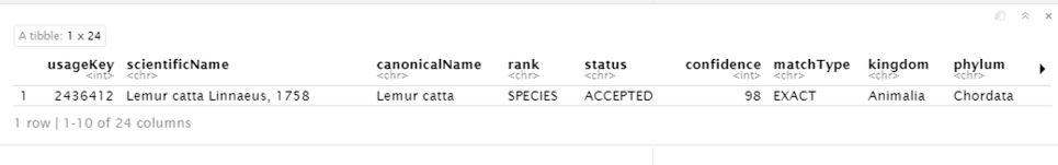
Looks like we have a good matched accepted name here. The usageKey is the key that identify the usage of a name in the GBIF Taxonomy Backbone. Once we decide which 'usage' is what we are looking for, We will use the key as the taxonKey for specifying the taxon for its occurrence data.
The following code block store the usageKey of Lemur catta in a variable usageKey.
usageKey <- 2436412
# Alternatively, since we know there is only one match, the following line will store the key in the variable, too.
# usageKey <- name_backbone(name = "Lemur catta", rank = "species") %>% pull(usageKey)
Use the taxonKey to generate the occurrence download of the species of interest
The following code block sends a request for download to the GBIF Occurrence API. A successful request will return a download key and initiate the preparing of the requested data. Note that as we’ve stored the key in the usageKey variable, for the required taxonKey for occ_download(), we simply supply the variable. Also, we need to supply our GBIF.org login credentials to request a download.
gd_key <- occ_download(
    pred("taxonKey", usageKey),
#   pred("hasCoordinate", TRUE),
    format = "SIMPLE_CSV",
    user = "USERNAME",
    pwd = "PASSWORD",
    email = "EMAIL_ADDRESS"
)
Note that, with "pred("hasCoordinate", TRUE),", we only want data with coordinates, which are required for our plotting. But you can test run the block with the line commented and see some errors would appear in later steps.
Once the download request is accepted, GBIF API will return a message with a download ID, which is then stored in gd_key.
Actually downloading the file
The download may take some time to prepare depending on the size. So it’s always good to fine tune the previous call to download only needed records. Once it’s ready, the download key can be used to retrieve the ZIP file and load the records, hence the following code block.
occ_download_wait(gd_key)

gd <- occ_download_get(gd_key, overwrite = TRUE) %>%
    occ_download_import()

head(gd, 10) # view first ten rows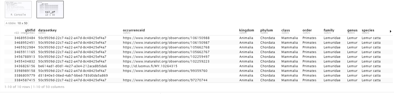
Data Visualization
Lemur catta is native to Madagascar; but just to make sure, let’s verify the data by plotting occurrences on a map.
ggplot() +
  geom_sf(data = world_map) +
  geom_point(data = gd,
             aes(x = decimalLongitude,
                 y = decimalLatitude),
             shape = "+",
             color = "red") +
  theme_bw()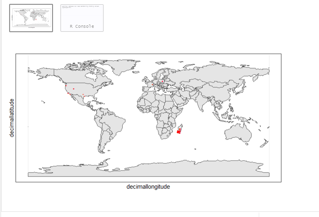
From the first look, is there anything unusual with the distribution of the Lemur species?
Whoops! It seems like there are unusual occurrences outside its native range. There are red dots dropped in other countries. We need to look into the data.
Also, we have a warning saying that some hundred rows of records contain missing values and are removed from the map. We should remove those first.
The following code block filters away records without decimallatitude or decimallongitude, then store the result as a new data frame gdf.
gdf <- gd %>% filter(!is.na(decimalLatitude), !is.na(decimalLongitude))We will from now on use gdf for our plotting. Let’s get back to the previous map and look at countries that have our data points.
table(gdf$countryCode)
It appears that many records have coordinates outside Madagascar. Let’s also have a look at the nature of these records.
gdf %>% distinct(basisOfRecord)
gdf %>% distinct(establishmentMeans)
There are 5 distinct values for DwC:basisOfRecord. We also looked at dwc:establishmentMeans, where only NATIVE is noted for some records.
Data cleaning
After some exploring of our data, we know that there are potential quality issues in our download. Apparently points outside Madagascar are suspicious, and we have just looked at basisOfRecord and establishmentMeans columns for cues of needed data actions.
Data cleaning typically involves procedures to remove unwanted records based on some criteria, or to correct values to achieve overall operable consistency. In the following section we will try to filter data, show the difference, and plot it on the map.
Step 1: basisOfRecord
We would like to evaluate observations and collections, so FOSSIL_SPECIMEN and MATERIAL_SAMPLE is not our concern here, let’s try to exclude them from our download.
clean_step1 <- gdf %>%
  as_tibble() %>%
  filter(!basisOfRecord %in% c("FOSSIL_SPECIMEN", "MATERIAL_SAMPLE"))

print(paste0(nrow(gdf)-nrow(clean_step1), " records deleted; ",
             nrow(clean_step1), " records remaining."))
Plotting raw records vs. cleaned records
We can use geom_point() multiple times to stack markers from different data frames. Here we show the cleaned records in red, and the raw ones in black. Notice the black marker "+" in Denmark(DK).
ggplot() +
  geom_sf(data = world_map) +
  geom_point(data = gdf,
             aes(x = decimalLongitude,
                 y = decimalLatitude),
             shape = "+",
             color = "black") +
  geom_point(data = clean_step1,
             aes(x = decimalLongitude,
                 y = decimalLatitude),
             shape = "+",
             color = "red") +
  theme_bw()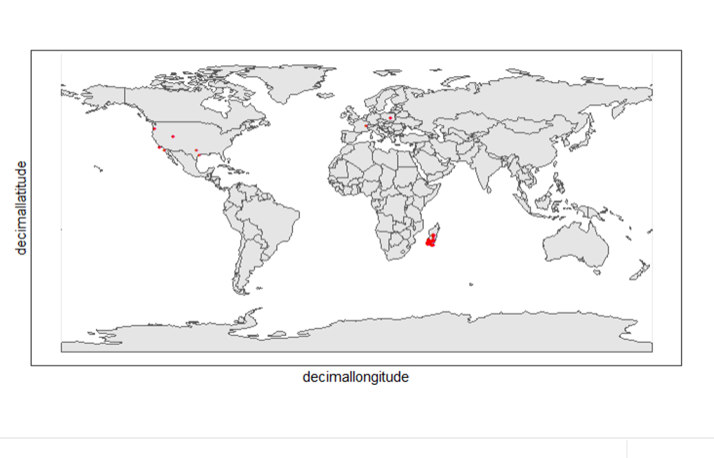
Step 2: Flagging problematic coordinates
Flagging records with problematic occurrence information using functions of the coordinateCleaner package. See comments for what each function does.
clean_step2 <- clean_step1 %>%
  filter(!is.na(decimalLatitude),
         !is.na(decimalLongitude),
         countryCode == "MG") %>% # "MG" is the ISO 3166-1 alpha-2 code for Madagascar
  cc_dupl() %>% # Identify duplicated records
  cc_zero() %>% # Identify zero coordinates
  cc_equ() %>% # Identify records with identical lat/lon
  cc_val() %>% # Identify invalid lat/lon coordinates
  cc_sea() %>% # Identify non-terrestrial coordinates
  cc_cap(buffer = 2000) %>% # Identify coordinates in vicinity of country capitals
  cc_cen(buffer = 2000) %>% # Identify coordinates in vicinity of country and province centroids
  cc_gbif(buffer = 2000) %>% # Identify records assigned to GBIF headquarters
  cc_inst(buffer = 2000) # Identify records in the vicinity of biodiversity institutions

print(paste0(nrow(gdf)-nrow(clean_step2), " records deleted; ",
             nrow(clean_step2), " records remaining."))
Plotting raw records vs. cleaned records (step 2)
ggplot() +
  geom_sf(data = world_map) +
  geom_point(data = gdf,
             aes(x = decimalLongitude,
                 y = decimalLatitude),
             shape = "+",
             color = "black") +
  geom_point(data = clean_step2,
             aes(x = decimalLongitude,
                 y = decimalLatitude),
             shape = "+",
             color = "red") +
  theme_bw()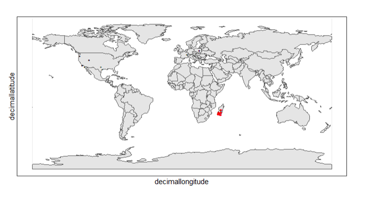
Again, the black "" markers indicate the occurrences of the raw dataset; whereas the red "" markers indicate the occurrences of the cleaned dataset.
Zooming in to madagascar
With cord_sf(), we can zoom in to show markers in Madagascar.
ggplot() +
  geom_sf(data = country_map) +
  geom_point(data = gdf,
             aes(x = decimalLongitude,
                 y = decimalLatitude),
             shape = "+",
             color = "black") +
  geom_point(data = clean_step2,
             aes(x = decimalLongitude,
                 y = decimalLatitude),
             shape = "+",
             color = "red") +
  coord_sf(xlim = st_bbox(country_map)[c(1,3)],
           ylim = st_bbox(country_map)[c(2,4)]) +
  theme_bw()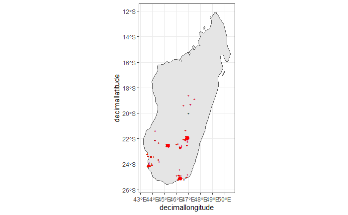
Step 3: Coordinate quality
We would like to further remove records with coordinate uncertainty and precision issues. The coordinate uncertainty in meters should be below 10000, and the coordinate precision should be better than 0.01.
clean_step3 <- clean_step2 %>%
  filter(is.na(coordinateUncertaintyInMeters) |
           coordinateUncertaintyInMeters < 10000,
         is.na(coordinatePrecision) |
           coordinatePrecision > 0.01)

print(paste0(nrow(gdf)-nrow(clean_step3), " records deleted; ",
             nrow(clean_step3), " records remaining." ))
We only have 14 records left, as shown in the following plot.
Plotting raw records vs. cleaned records (step 3)
ggplot() +
  geom_sf(data = country_map) +
  geom_point(data = gdf,
             aes(x = decimalLongitude,
                 y = decimalLatitude),
             shape = "+",
             color = "black") +
  geom_point(data = clean_step3,
             aes(x = decimalLongitude,
                 y = decimalLatitude),
             shape = "+",
             color = "red") +
  coord_sf(xlim = st_bbox(country_map)[c(1,3)],
           ylim = st_bbox(country_map)[c(2,4)]) +
  theme_bw()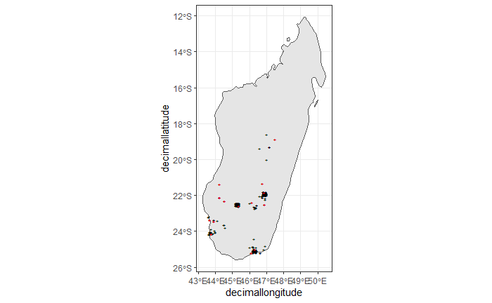
Step 4: Temporal range filtering
We might have other data layers to work with the occurrence download (e.g. WorldClim provides data from 1960). Depending on the temporal availability of the data, say, only after 1955, we also want to filter away occurrence records prior to the year as it wouldn’t be used.
The filter() function applying to temporal attributes can easily remove records with temporal range outside that of our predictor variables.
clean_step4 <- clean_step3 %>%
  filter(year >= 1955)

print(paste0(nrow(gdf)-nrow(clean_step3), " records deleted; ",
             nrow(clean_step4), " records remaining." ))
As a result, we have only three records after applying this filter. See the next plot.
ggplot() +
  geom_sf(data = country_map) +
  geom_point(data = gdf,
             aes(x = decimalLongitude,
                 y = decimalLatitude),
             shape = "+",
             color = "black") +
  geom_point(data = clean_step4,
             aes(x = decimalLongitude,
                 y = decimalLatitude),
             shape = "+",
             color = "red") +
  coord_sf(xlim = st_bbox(country_map)[c(1,3)],
           ylim = st_bbox(country_map)[c(2,4)]) +
  theme_bw()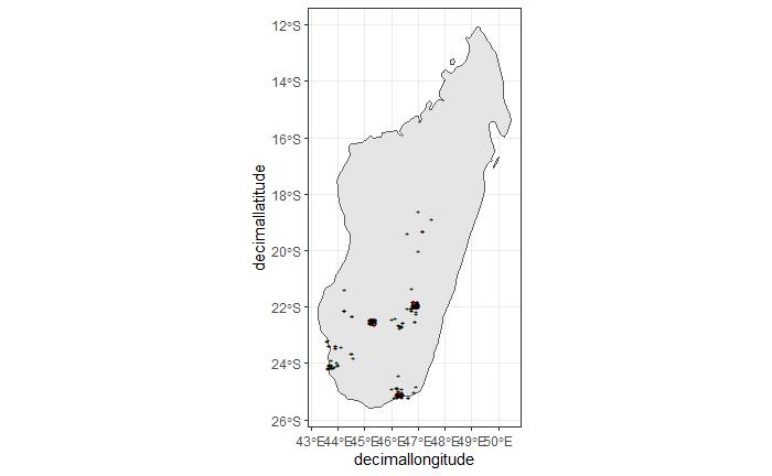
Conclusion
This document merely demonstrates what GBIF data users could do after downloading data from the global index. Before feeding data into an analytic workflow, users usually examine the download by looking at unique values and visualising facets and then decide to clean or filter the data so that the subsequent analysis can run with desired settings. The process can include many trials and adjustments, and here, we have introduced some of them.